⭐文章目录⭐
👇
Backtracking
Backtracking is a general algorithmic technique for solving problems incrementally, where you build candidates for the solution step by step, and abandon (“backtrack”) a candidate as soon as you determine it cannot lead to a valid solution.
An example:
DFS()
- What makes the time complexity analysis of a backtracking algorithm very difficult is that the number of solutions that do satisfy the restriction is hard to estimate.
N-Queens Problem
- Put N queens on an N x N chessboard.
- No two Queens can attack each other(in the same row,col or diagonal).
Fact
- For a $N>3$,a feasible solution exists.
- For some special $N$($N$ is prime or $6k+1$), a solution can be efficiently found.
Backtracking Approach
- 1.Construct a game tree like the following:
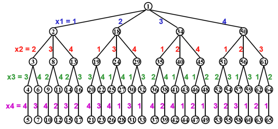
- 2.Start from the root node and explore all possible moves,for example:
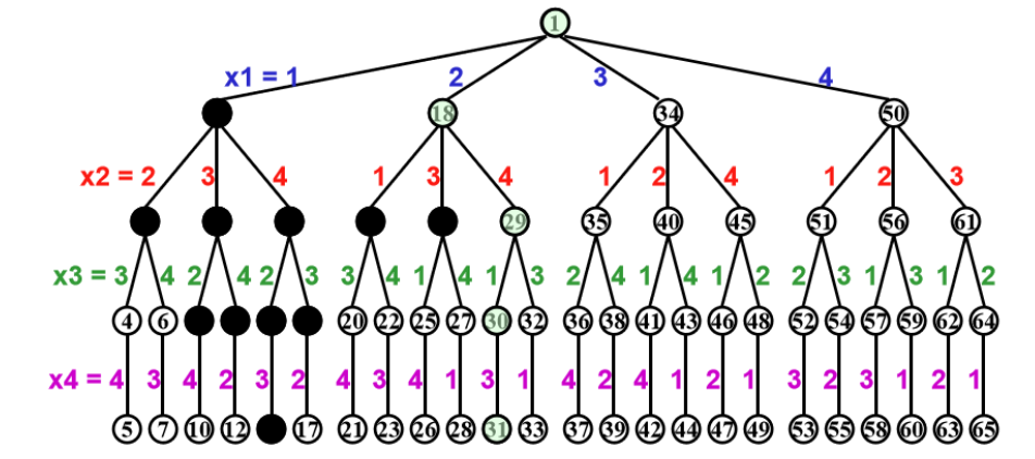
for i in range(N):
    p[i]=-1
i=0
while 0 <= i < N:
    findgood=false
    for j in range(p[i]+1,N):
        if j not aattack P[0],P[1]...P[j-1]
            p[i]=j
            findgood=true
            break
    if findgood:
        i=i+1
    else:
        i--
if i==-1:
    not found
if i==N:
    found
This algorithm takes $O(N!N)$ time to solve the problem.
Turnpike Problem
- Given a set $A$ of points on a line, $D(A) =$ {|$a-b$|$|$ for all $a,b\in A$}
- Now given a set D ,we need to find a set $A$ such that $D(A) = D$.
Backtracking Approach
- 1.Compute out the number of points
- 2.Set $x_0$ as 0, and $x_{max}$ as $max(D)$
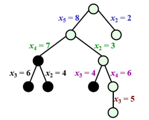
- 3.Find the last largest $x_i$ in $D$, and there is only two cases:
- case 1: $x_{max}-x_i$
- case 2: $x_i$
- 4.Then construct a game tree like the following:
TP(D,A):
if D is empty:
    return True
d=max(D)
for a' in {d,a_max-d}:
    delta={|a'-a|,a in A}
    if delta in D:
        delete(D,delta)
        A=A+{a'}
        if TP(D,A):
            return True
        else:
            A=A-{a'}
            insert(D,delta)
return False
This algorithm takes $O(nlogn)$ time to compute each node.And the total time complexity is $O(n)$in the best case,but it can be $O(2^n)$ in the worst case.
Pruning
Pruning is a technique used to reduce the number of branches in a search tree. It is used to reduce the search space and improve the efficiency of the search algorithm.
We first consider a problem like this:
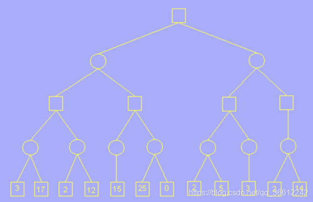
- In the picture above, we have a decision tree and each leaf is a result of decisions.
- For a circle node, we always choose the case that minimize the result.
- For a square node, we always choose the case that maximize the result.
- We define $\alpha$ and $\beta$ as the current best and worst result of current situation.And they are initialized as $-\infty$ and $\infty$ respectively.
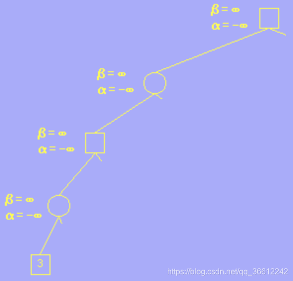
- Then we go through each leaf node and update like this:
- 1.Circle meets 3, $3<\beta=\infty$,so we update $\beta=3$.
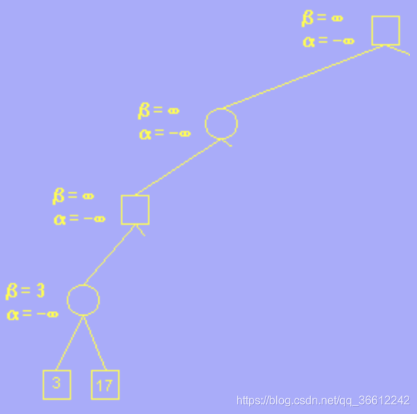
- 2.Circle meets 17, $17>\beta=3$,so we do not update $\beta$.
- 3.square meets 3, $3>\alpha=-\infty$,so we update $\alpha=3$.
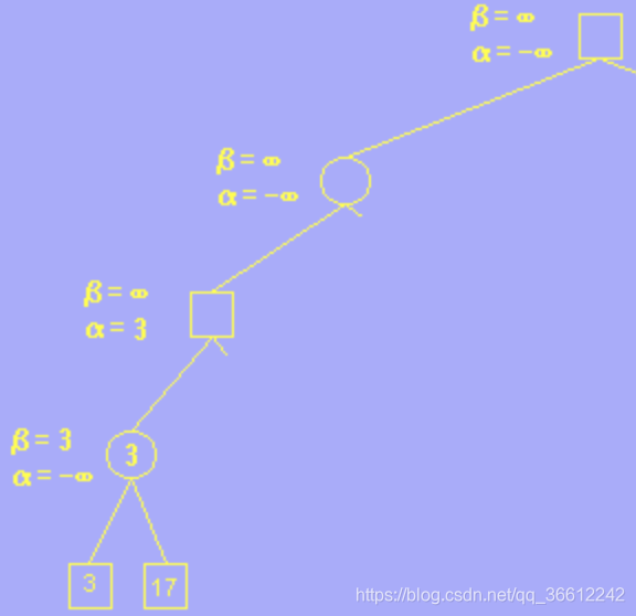
- 4.Circle meets 2, its $\alpha$ and $\beta$ is the same of its parent.And $2<\beta=\infty$,so we update $\beta=2$.
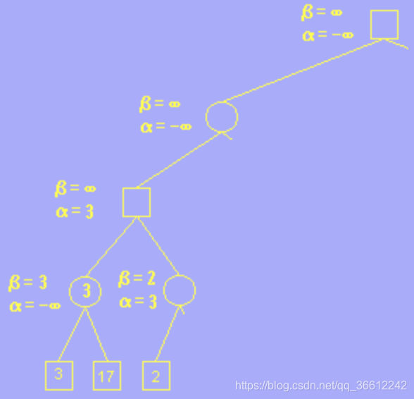
- 5 .As for a circle node, if its $\beta<\alpha$,this means that its parent square node will not choose it due to the fact that:
- 1.Circle will choose a result no larger than $\beta=2$.
- 2.square will choose a result no less than $\alpha=3$.
- 6 .So we can prune the remained ,unaccessed node of this circle node,which is called $\alpha$-pruning.
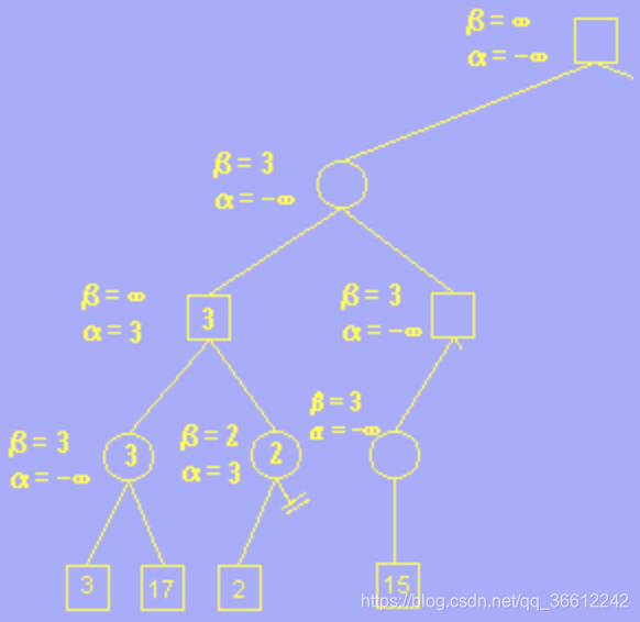
- 7.And then we go through like how we did before until we meet this situation:
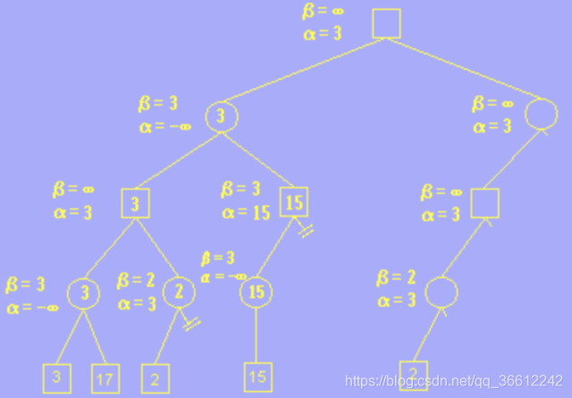
- 8.For a square node, if its $\alpha>\beta$,this means that its parent circle node will not choose it due to the same reason.
- 9 .So we can prune the remained ,unaccessed node of this square node,which is called $\beta$-pruning.
